- Click a cell in the source data or table range.
- Go to Insert > Recommended PivotTable.
- Excel analyzes your data and presents you with several options, like in this example using the household expense data.
- Select the PivotTable that looks best to you and press OK.
How do I generate a pivot table?
To create the Pivot Table and apply conditional formatting, you need to perform the following steps:
- Click anywhere in the data.
- Go to Insert > Recommended PivotTables. Scroll down and select the one that says Sum of Sales by Items and Month.
- Click OK.
How do you insert a formula in a pivot table?
- In the Power Pivot window, Click Home> View> Calculation Area.
- Click on an empty cell in the Calculation Area.
- In the formula bar, at the top of the table, enter the formula, % of wins := DIVIDE (CALCULATE (COUNTA ( [Win]),FILTER (Table1,Table1 [Win]="Y")),COUNTA ( [Name]),0)
- Press Enter to accept the formula.
- Click anywhere in the Power Pivot data. ...
How to quickly format a pivot table?
Pivot Table Formatting
- Default Style Options. There are a few options available on the ribbon once you have pivot table on your worksheet. ...
- Change Pivot Table Formatting. Now to choose a particular style as a default for your PivotTables use the following steps. ...
- Duplicate and Modify. ...
- Copy Layout to a Different Worksheet. ...
- More on Pivot Table
How to set up Excel pivot table for beginners?
Pivot Tables
- Insert a Pivot Table. To insert a pivot table, execute the following steps. ...
- Drag fields. The PivotTable Fields pane appears. ...
- Sort. To get Banana at the top of the list, sort the pivot table. ...
- Filter. Because we added the Country field to the Filters area, we can filter this pivot table by Country. ...
- Change Summary Calculation. ...
- Two-dimensional Pivot Table. ...
Where is the recommended pivot tables in Excel?
Insert tabTo create a recommended PivotTable from the data, I click any cell in the list, and then on the Insert tab, click Recommended PivotTables. Doing so displays the Recommended PivotTables dialog box. I can scroll down the list of recommendations, and the one that's selected is previewed here in the right-hand pane.
How do I create a shortcut key for a PivotTable?
To insert a new pivot table, simply select any cell in your data set and press the shortcut keys ALT + N + V. This will open the Insert PivotTable dialog box, where you can choose where to place the new pivot table.
How do you insert the sum of total by Sales type recommended PivotTable?
Click on COUNT of SALES and select Value Field Settings. We want it to display the Total sum of Sales per Product instead. Select Sum and click OK. With just that, your Pivot Table is now ready!
What is the easiest way to add a PivotTable to your spreadsheet?
On the Home tab, select PivotTable. Select where you want the PivotTable to be placed: a new worksheet, or the current location. Click OK, and Excel will add an empty PivotTable with the Field List pane displayed on the right.
What is the formula for pivot table in Excel?
This displays the PivotTable Tools, adding the Analyze and Design tabs. On the Analyze tab, in the Calculations group, click Fields, Items, & Sets, and then click Calculated Field. In the Name box, select the calculated field for which you want to change the formula. In the Formula box, edit the formula.
How do I create a pivot table in Excel with multiple columns?
To have multiple columns: Click in one of the cells of your pivot table. Click your right mouse button and select Pivot table Options in the context menu, this will open a form with tabs. Click on the tab Display and tag the check box Classic Pivot table layout.
How do I add grand totals to a pivot table in Excel?
Click anywhere in the PivotTable. On the Design tab, in the Layout group, click Grand Totals, and then select the grand total display option that you want.
How do you add a total to a table automatically?
Total the data in an Excel tableClick anywhere inside the table.Go to Table Tools > Design, and select the check box for Total Row.The Total Row is inserted at the bottom of your table. ... Select the column you want to total, then select an option from the drop-down list.
How do I add a custom subtotal to a pivot table?
To create a custom subtotal:Right-click a label for the field in which you want to change the subtotal. ... In the pop-up menu, click Field Settings.In the Field Settings dialog box, click the Subtotals & Filters tab.Under Subtotals, click Custom.In the list of Summary Functions, click one or more function names.More items...•
How do I add a pivot table to a spreadsheet?
Add a pivot table from a suggestionIn Sheets, open your spreadsheet that contains the source data.At the bottom right, click Explore .Scroll down to the Pivot Table section to see suggested pivot tables. Click More to see additional suggestions. ... Hover over the pivot table you want and click Insert pivot table .
How do I automatically add data to a pivot table?
Refresh data automatically when opening the workbookClick anywhere in the PivotTable to show the PivotTable Tools on the ribbon.Click Analyze > Options.On the Data tab, check the Refresh data when opening the file box.
What data do you need for a pivot table?
Conditions to Create a Pivot TableEach column of the Pivot Table must have a title.The title should be written in a single row.In a column, all the items should be of the same data type (numbers, dates or strings).The data table should not contain any merged cells.More items...
Can you create a shortcut key in Excel?
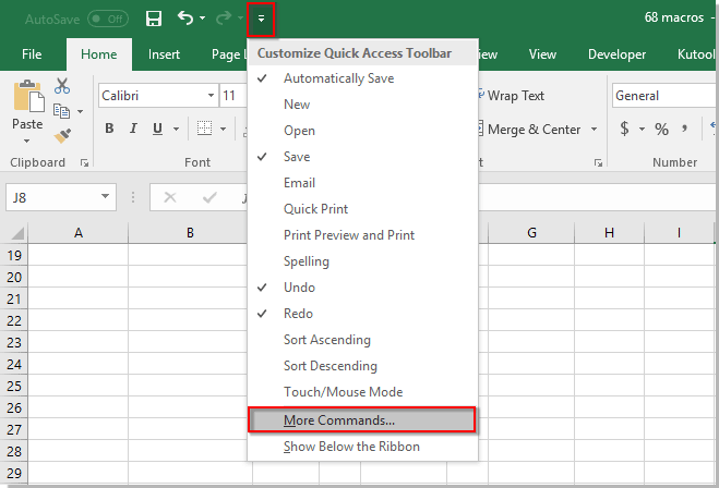
Use a mouse to assign or remove a keyboard shortcut Go to File > Options > Customize Ribbon. At the bottom of the Customize the Ribbon and keyboard shortcuts pane, select Customize. In the Save changes in box, select the current document name or template that you want to save the keyboard shortcut changes in.
How do I assign a quick key?
0:141:35How to Assign Shortcut Keys on a PC - YouTubeYouTubeStart of suggested clipEnd of suggested clipYou will need a PC the desire to save time and a list of shortcuts. Step 1 locate the fileMoreYou will need a PC the desire to save time and a list of shortcuts. Step 1 locate the file application or folder that you would like to gain faster access to step 2 right-click on the file. And then
How do I add a shortcut to a table?
6. Want to insert a table, row, column, comment, or chart? Press Ctrl + l to insert a table, Ctrl + Shift + + to insert a cell, row, or column, Ctrl + F2 to insert a comment, and Alt + F1 to insert a chart with data. 7.
How do you create a table shortcut?
Insert a Table. Turning your data into an Excel Table is really easy when you use the shortcut Ctrl + T .
How to add a field to a pivot table?
To add a field to your PivotTable, select the field name checkbox in the PivotTables Fields pane.
What is pivot table?
PivotTables are great ways to summarize, analyze, explore, and present summary data, and in Excel for the web you can also collaborate with someone on a PivotTable at the same time.
How to insert a pivot table in Excel?
Insert a Pivot Table. To insert a pivot table, execute the following steps. 1. Click any single cell inside the data set. 2. On the Insert tab, in the Tables group, click PivotTable. The following dialog box appears. Excel automatically selects the data for you.
What is pivot table?
Pivot tables are one of Excel 's most powerful features. A pivot table allows you to extract the significance from a large, detailed data set.
How to change pivot table data?
If you simply want to change the data in your pivot table, alter the data here. Go back to the pivot table tab. Click the tab on which your pivot table is listed. Select your pivot table. Click the pivot table to select it. Click the Analyze tab.
How to open pivot table in Excel?
1. Open your pivot table Excel document. Double-click the Excel document that contains your pivot table. It will open. ...
Where is the analyze tab in Excel?
Click the Analyze tab. It's in the middle of the green ribbon that's at the top of the Excel window. Doing so will open a toolbar just below the green ribbon.
Where is the refresh button in pivot table?
While in the data of the Pivot Table, the Analyze/Design tabs are viewable on the Ribbon, select the 'Refresh' button on the ribbon (it has 2 arrows that create a circle).
Can you add data to a pivot table?
This wikiHow teaches you how to add data to an existing pivot table in Microsoft Excel. You can do this in both Windows and Mac versions of Excel.
How to insert pivot table in Excel?
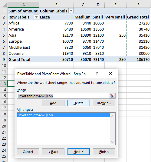
Start the Pivot Table wizard. Click the "Insert" tab at the top of the Excel window. Click the "PivotTable" button on the left side of the Insert ribbon. If you are using Excel 2003 or earlier, click the Data menu and select PivotTable and PivotChart Report...
What is pivot table?
As the word pivot means revolving around a hinge, the same is case with pivot tables . In simple words, it creates dynamic fields which we can operate as we want. For example, we want to make any column into row, just drag it, we want to do total, average , count, just do it in a click. This makes using the document less time consuming.
How do pivot tables work?
Pivot tables are interactive tables that allow the user to group and summarize large amounts of data in a concise, tabular format for easier reporting and analysis. They can sort, count, and total the data, and are available in a variety of spreadsheet programs. Excel allows you to easily create pivot tables by dragging and dropping your relevant information into the appropriate boxes. You can then filter and sort your data to find patterns and trends.
How to switch pivot table back and forth?
By default, Excel will place the table on a new worksheet, allowing you to switch back and forth by clicking the tabs at the bottom of the window.
How many columns should be in a pivot table?
This basically just means that at least one column should have repeating data.
Can you add multiple fields to a pivot table?
Add multiple fields to a section. Pivot tables allow you to add multiple fields to each section, allowing for more minute control over how the data is displayed. Using the above example, say you make several types of tables and several types of chairs. Your spreadsheet is records whether the item is a table or chair (Product Type), but also the exact model of the table or chair sold (Model).
Does pivot table update?
Update your spreadsheet. Your pivot table will automatically update as you modify the base spreadsheet. This can be great for monitoring your spreadsheets and tracking changes. .
Insert A Pivot Table

Drag Fields
- The PivotTable Fields paneappears. To get the total amount exported of each product, drag the following fields to the different areas. 1. Product field to the Rows area. 2. Amount field to the Values area. 3. Country field to the Filters area. Below you can find the pivot table. Bananas are our main export product. That's how easy pivot tables can be!
Sort
- To get Banana at the top of the list, sort the pivot table. 1. Click any cell inside the Sum of Amount column. 2. Right click and click on Sort, Sort Largest to Smallest. Result.
Filter
- Because we added the Country field to the Filters area, we can filter this pivot table by Country. For example, which products do we export the most to France? 1. Click the filter drop-down and select France. Result. Apples are our main export product to France. Note: you can use the standard filter (triangle next to Row Labels) to only show the amounts of specific products.
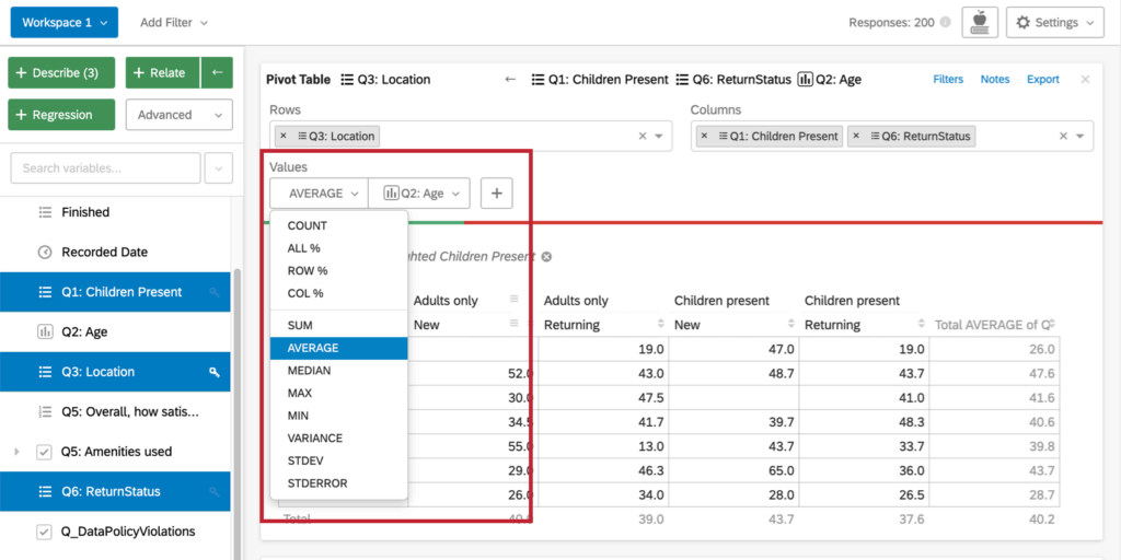
Change Summary Calculation
- By default, Excel summarizes your data by either summing or counting the items. To change the type of calculation that you want to use, execute the following steps. 1. Click any cell inside the Sum of Amount column. 2. Right click and click on Value Field Settings. 3. Choose the type of calculation you want to use. For example, click Count. 4. Click OK. Result. 16 out of the 28 order…
Two-Dimensional Pivot Table
- If you drag a field to the Rows area and Columns area, you can create a two-dimensional pivot table. First, insert a pivot table. Next, to get the total amount exported to each country, of each product, drag the following fields to the different areas. 1. Country field to the Rows area. 2. Product field to the Columns area. 3. Amount field to the Values area. 4. Category field to the Filt…