
Full Answer
What are some of the limitations of principal component analysis?
Disadvantages of Principal Component Analysis. 1. Independent variables become less interpretable: After implementing PCA on the dataset, your original features will turn into Principal Components. Principal Components are the linear combination of your original features. Principal Components are not as readable and interpretable as original ...
Which software is suitable to do PCA analysis?
you can find QStudioMetrics, an opensource software for multivariate analysis. The software It is able to run PCA/PLS using the NIPALS algorithm. Moreover it is able to run Linear Discriminant Analysis and Multiple Linear Regression. The software runs under graphical user interface and it process CSV as well as TXT input files.
How to analyse data using SPSS?
Steps
- Load your excel file with all the data. Once you have collected all the data, keep the excel file ready with all data inserted using the right tabular forms.
- Import the data into SPSS. You need to import your raw data into SPSS through your excel file. ...
- Give specific SPSS commands. ...
- Retrieve the results. ...
- Analyse the graphs and charts. ...
What is principal components analysis (PCA)?
Principal component analysis (PCA) is a mathematical algorithm that reduces the dimensionality of the data while retaining most of the variation in the data set 1. It accomplishes this reduction by identifying directions, called principal components, along which the variation in the data is maximal.
What does a principal component analysis tell you?
Principal component analysis, or PCA, is a statistical procedure that allows you to summarize the information content in large data tables by means of a smaller set of “summary indices” that can be more easily visualized and analyzed.
What do principal components tell us?
Geometrically speaking, principal components represent the directions of the data that explain a maximal amount of variance, that is to say, the lines that capture most information of the data.
What is principal component analysis explain with an example?
Principal Component Analysis is an unsupervised learning algorithm that is used for the dimensionality reduction in machine learning. It is a statistical process that converts the observations of correlated features into a set of linearly uncorrelated features with the help of orthogonal transformation.
What does PC1 and PC2 mean?
Most of the variability in the data is captured by PC1 (Principal Component 1) and the residual variability is captured by PC2 (Principal Component 2), which is orthogonal (independent) to PC1. PC2 tries to capture the abnormal variations in the dataset. PC1 and PC2 have 0 correlation.
When should we use PCA?
PCA should be used mainly for variables which are strongly correlated. If the relationship is weak between variables, PCA does not work well to reduce data. Refer to the correlation matrix to determine. In general, if most of the correlation coefficients are smaller than 0.3, PCA will not help.
What type of data is good for PCA?
PCA works best on data set having 3 or higher dimensions. Because, with higher dimensions, it becomes increasingly difficult to make interpretations from the resultant cloud of data. PCA is applied on a data set with numeric variables. PCA is a tool which helps to produce better visualizations of high dimensional data.
How PCA works step by step?
ImplementationStep 1: Create random data. ... Step 2: Mean Centering/ Normalize data. ... Step 3: Compute the covariance matrix. ... Step 4: Compute eigen vectors of the covariance matrix. ... Step 5: Compute the explained variance and select N components. ... Step 6: Transform Data using eigen vectors.More items...•
What is the main purpose of principal component analysis in machine learning?
The Principal Component Analysis is a popular unsupervised learning technique for reducing the dimensionality of data. It increases interpretability yet, at the same time, it minimizes information loss. It helps to find the most significant features in a dataset and makes the data easy for plotting in 2D and 3D.
What is the difference between PCA and factor analysis?
PCA is used to decompose the data into a smaller number of components and therefore is a type of Singular Value Decomposition (SVD). Factor Analysis is used to understand the underlying 'cause' which these factors (latent or constituents) capture much of the information of a set of variables in the dataset data.
How do you interpret the principal component analysis in SPSS?
The steps for interpreting the SPSS output for PCALook in the KMO and Bartlett's Test table.The Kaiser-Meyer-Olkin Measure of Sampling Adequacy (KMO) needs to be at least . 6 with values closer to 1.0 being better.The Sig. ... Scroll down to the Total Variance Explained table. ... Scroll down to the Pattern Matrix table.
What is PC1 and PC2 and PC3?
What does PC stands for? Profit Contribution 1 (PC1) Profit Contribution 2 (PC2) Profit Contribution 3 (PC3) Conclusion.
How do you read PCoA plots?
Interpretation of a PCoA plot is straightforward: objects ordinated closer to one another are more similar than those ordinated further away. (Dis)similarity is defined by the measure used in the construction of the (dis)similarity matrix used as input.
What is principal component?
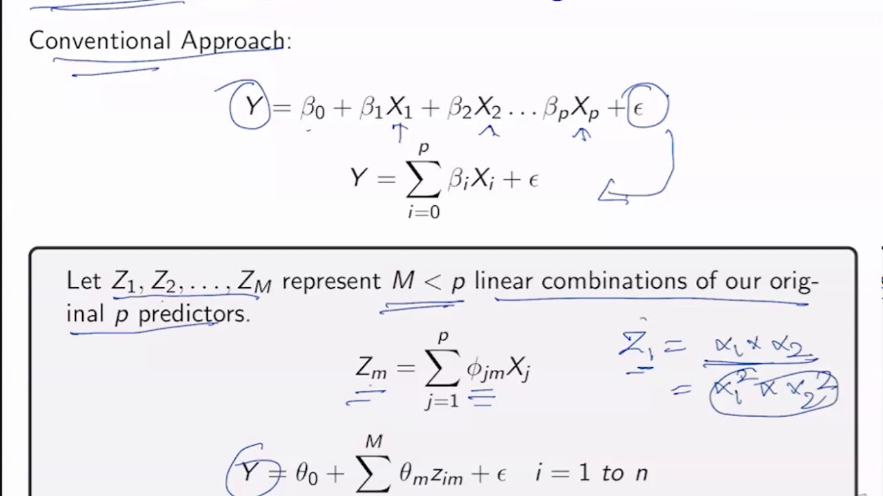
Principal components are new variables that are constructed as linear combinations or mixtures of the initial variables. These combinations are done in such a way that the new variables (i.e., principal components) are uncorrelated and most of the information within the initial variables is squeezed or compressed into the first components. So, the idea is 10-dimensional data gives you 10 principal components, but PCA tries to put maximum possible information in the first component, then maximum remaining information in the second and so on, until having something like shown in the scree plot below.
How many steps are there in principal component analysis?
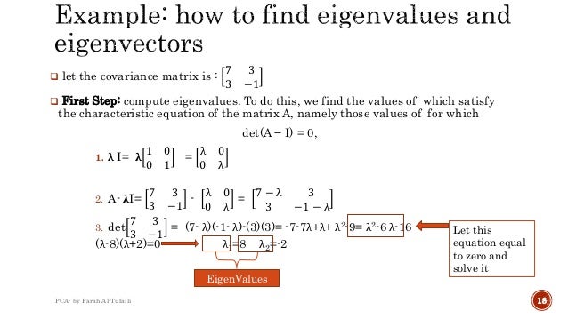
Principal component analysis can be broken down into five steps. I'll go through each step, providing logical explanations of what PCA is doing and simplifying mathematical concepts such as standardization, covariance, eigenvectors and eigenvalues without focusing on how to compute them.
How to do a PCA?
How do you do a PCA? 1 Standardize the range of continuous initial variables 2 Compute the covariance matrix to identify correlations 3 Compute the eigenvectors and eigenvalues of the covariance matrix to identify the principal components 4 Create a feature vector to decide which principal components to keep 5 Recast the data along the principal components axes
What is PCA in data analysis?
So to sum up, the idea of PCA is simple — reduce the number of variables of a data set, while preserving as much information as possible.
What is the eigenvector that corresponds to the first principal component?
If we rank the eigenvalues in descending order, we get λ1>λ2, which means that the eigenvector that corresponds to the first principal component (PC1) is v1 and the one that corresponds to the second component (PC2) is v2.
What is PCA in statistics?
Principal Component Analysis, or PCA, is a dimensionality-reduction method that is often used to reduce the dimensionality of large data sets, by transforming a large set of variables into a smaller one that still contains most of the information in the large set.
What is the first step in PCA?
Step 1: Standardization . The aim of this step is to standardize the range of the continuous initial variables so that each one of them contributes equally to the analysis. More specifically, the reason why it is critical to perform standardization prior to PCA, is that the latter is quite sensitive regarding the variances of the initial variables.
What is the purpose of principal components analysis?
A variant of principal components analysis is used in neuroscience to identify the specific properties of a stimulus that increase a neuron 's probability of generating an action potential. This technique is known as spike-triggered covariance analysis. In a typical application an experimenter presents a white noise process as a stimulus (usually either as a sensory input to a test subject, or as a current injected directly into the neuron) and records a train of action potentials, or spikes, produced by the neuron as a result. Presumably, certain features of the stimulus make the neuron more likely to spike. In order to extract these features, the experimenter calculates the covariance matrix of the spike-triggered ensemble, the set of all stimuli (defined and discretized over a finite time window, typically on the order of 100 ms) that immediately preceded a spike. The eigenvectors of the difference between the spike-triggered covariance matrix and the covariance matrix of the prior stimulus ensemble (the set of all stimuli, defined over the same length time window) then indicate the directions in the space of stimuli along which the variance of the spike-triggered ensemble differed the most from that of the prior stimulus ensemble. Specifically, the eigenvectors with the largest positive eigenvalues correspond to the directions along which the variance of the spike-triggered ensemble showed the largest positive change compared to the variance of the prior. Since these were the directions in which varying the stimulus led to a spike, they are often good approximations of the sought after relevant stimulus features.
How is factor analysis different from PCA?
Different from PCA, factor analysis is a correlation-focused approach seeking to reproduce the inter-correlations among variables, in which the factors "represent the common variance of variables, excluding unique variance". In terms of the correlation matrix, this corresponds with focusing on explaining the off-diagonal terms (that is, shared co-variance), while PCA focuses on explaining the terms that sit on the diagonal. However, as a side result, when trying to reproduce the on-diagonal terms, PCA also tends to fit relatively well the off-diagonal correlations. : 158 Results given by PCA and factor analysis are very similar in most situations, but this is not always the case, and there are some problems where the results are significantly different. Factor analysis is generally used when the research purpose is detecting data structure (that is, latent constructs or factors) or causal modeling. If the factor model is incorrectly formulated or the assumptions are not met, then factor analysis will give erroneous results.
What are the disadvantages of PCA?
A particular disadvantage of PCA is that the principal components are usually linear combinations of all input variables. Sparse PCA overcomes this disadvantage by finding linear combinations that contain just a few input variables. It extends the classic method of principal component analysis (PCA) for the reduction of dimensionality of data by adding sparsity constraint on the input variables. Several approaches have been proposed, including
Why is PCA important?
Spike sorting is an important procedure because extracellular recording techniques often pick up signals from more than one neuron. In spike sorting, one first uses PCA to reduce the dimensionality of the space of action potential waveforms, and then performs clustering analysis to associate specific action potentials with individual neurons.
What is PCA in math?
PCA is defined as an orthogonal linear transformation that transforms the data to a new coordinate system such that the greatest variance by some scalar projection of the data comes to lie on the first coordinate (called the first principal component), the second greatest variance on the second coordinate, and so on.
What is PCA in data analysis?
Principal component analysis ( PCA) is the process of computing the principal components and using them to perform a change of basis on the data, sometimes using only the first few principal components and ignoring the rest. PCA is used in exploratory data analysis and for making predictive models.
When was PCA invented?
PCA was invented in 1901 by Karl Pearson, as an analogue of the principal axis theorem in mechanics; it was later independently developed and named by Harold Hotelling in the 1930s. Depending on the field of application, it is also named the discrete Karhunen–Loève transform (KLT) in signal processing, the Hotelling transform in multivariate quality control, proper orthogonal decomposition (POD) in mechanical engineering, singular value decomposition (SVD) of X (invented in the last quarter of the 19th century ), eigenvalue decomposition (EVD) of XTX in linear algebra, factor analysis (for a discussion of the differences between PCA and factor analysis see Ch. 7 of Jolliffe's Principal Component Analysis ), Eckart–Young theorem (Harman, 1960), or empirical orthogonal functions (EOF) in meteorological science, empirical eigenfunction decomposition (Sirovich, 1987), empirical component analysis (Lorenz, 1956), quasiharmonic modes (Brooks et al., 1988), spectral decomposition in noise and vibration, and empirical modal analysis in structural dynamics.
Principal Component Analysis (PCA) Explained Visually with Zero Math
Principal Component Analysis (PCA) is an indispensable tool for visualization and dimensionality reduction for data science but is often buried in complicated math. It was tough-, to say the least, to wrap my head around the whys and that made it hard to appreciate the full spectrum of its beauty.
What is PCA?
Principal component analysis (PCA) is a technique that transforms high-dimensions data into lower-dimensions while retaining as much information as possible.
How does PCA work?
It’s a two-step process. We can’t write a book summary if we haven’t read or understood the content of the book.
The PC That Got Away
Since we’re not choosing all the principal components, we inevitably lose some information. But we haven’t exactly described what we are losing. Let’s dive deeper into that with a new toy example.
Implementing PCA in Python
There is much more to PCA beyond the premise of this article. The only way to truly appreciate the beauty of PCA is to experience it yourself. Hence, I would love to share some code snippets here for anyone that wants to get their hands dirty. The full code can be assessed here with Google Colab.
Final Remarks
PCA is a mathematically beautiful concept and I hope I was able to convey it in a casual tone so it doesn’t feel overwhelming. For those that are eager to look into the nitty-gritty details, I have attached some interesting discussions/resources below for your perusal.
Why does Principal Components Analysis Work?
This section dives into the mathematical details of principal components analysis. To be able to follow along, you should be familiar with the following mathematical topics. I’ve linked each topic to a corresponding post on this blog with an explanation of the topic.
Why are principal components important?
Practically speaking, principal components are feature combinations that represent the data and its differences as efficiently as possible by ensuring that there is no information overlap between features. The original features often display significant redundancy, which is the main reason why principal components analysis works so well at reducing dimensionality.
What is PCA in statistics?
Principal Components Analysis, also known as PCA, is a technique commonly used for reducing the dimensionality of data while preserving as much as possible of the information contained in the original data. PCA achieves this goal by projecting data onto a lower-dimensional subspace that retains most of the variance among the data points.
How much variance does the first two principal components capture?
It seems like the first two principal components capture almost 30% of the variance contained in the original 64-dimensional representation.
Why do data points cluster together?
This happens because you are explicitly focusing on axes that maximize the variance.
Can you project data points onto a line using PCA?
If you have data in a 2-dimensional space, you could project all the data points onto a line using PCA.
What is the purpose of principal components?
The primary objective of Principal Components is to represent the information in the dataset with minimum columns possible .
What is the object of pca.components_?
The pca.components_ object contains the weights (also called as ‘loadings’) of each Principal Component. It is using these weights that the final principal components are formed.
Why is PCA used?
Practically PCA is used for two reasons: Dimensionality Reduction: The information distributed across a large number of columns is transformed into principal components (PC) such that the first few PCs can explain a sizeable chunk of the total information (variance).
What is the name of the PCA module?
Using scikit-learn package, the implementation of PCA is quite straight forward. The module named sklearn.decomposition provides the PCA object which can simply fit and transform the data into Principal components.
What is PCA in math?
Principal Components Analysis (PCA) is an algorithm to transform the columns of a dataset into a new set of features called Principal Components. By doing this, a large chunk of the information across the full dataset is effectively compressed in fewer feature columns. This enables dimensionality reduction and ability to visualize the separation of classes or clusters if any.
Which method gives back the original data when you input principal components features?
The fitted pca object has the inverse_transform() method that gives back the original data when you input principal components features.
How to see how much of the total information is contributed by each PC?
To see how much of the total information is contributed by each PC, look at the explained_variance_ratio_ attribute.
Why are principal components important?
This is nice in several ways: Principal components help reduce the number of dimensions down to 2 or 3, making it possible to see strong patterns. Yet you didn’t have to throw away any genes in doing so. Principal components take all dimensions and data points into account.
What is PCA in biology?
Short for principal component analysis, PCA is a way to bring out strong patterns from large and complex datasets. For example, if you measure the expression of 15 genes from 60 mice, and the data come back as a 15×60 table, how do you make sense of all that? How do you even know which mice are similar to one another, and which ones are different? How do you know which genes are responsible for such similarities or differences?
What is PCA in statistics?
To sum up, principal component analysis (PCA) is a way to bring out strong patterns from large and complex datasets. The essence of the data is captured in a few principal components, which themselves convey the most variation in the dataset. PCA reduces the number of dimensions without selecting or discarding them.
How many genes are in a PCA?
PCA deals with the curse of dimensionality by capturing the essence of data into a few principal components. But we have 15 genes, not just 2. The more genes you’ve got, the more axes (dimensions) there are when you plot their expression.
How many directions does PCA rotate?
This is when the magic of PCA comes in. To create PC1, a line is anchored at the center of the 15-D cloud of dots and rotate in 15 directions, all the while acting as a “mirror,” on which the original 60 dots are projected.
What is PC1 in physics?
Principal component 1 (PC1) is a line that goes through the center of that cloud and describes it best. It is a line that, if you project the original dots on it, two things happen: The total distance among the projected points is maximum. This means they can be distinguished from one another as clearly as possible.
Which line must convey the maximum variation among data points and contain minimum error?
In other words, the best line — our PC1 — must convey the maximum variation among data points and contain minimum error. These two things are actually achieved at the same time, because Pythagoras said so.
What is principal component analysis?
Principal Component analysis is a form of multidimensional scaling. It is a linear transformation of the variables into a lower dimensional space which retain maximal amount of information about the variables. For example, this would mean we could look at the types of subjects each student is maybe more suited to.
How many principal component scores are there?
There are six principal component scores in the table above. You can now plot the scores in a 2D graph to get a sense of the type of subjects each student is perhaps more suited to.
What is PCA in statistics?
Principal component analysis (PCA) is one popular approach analyzing variance when you are dealing with multivariate data. You have random variables X1, X2,...Xn which are all correlated (positively or negatively) to varying degrees, and you want to get a better understanding of what's going on. PCA can help.
What are the components of a data matrix?
The principal components of a data matrix are the eigenvector-eigenvalue pairs of its variance-covariance matrix. In essence, they are the decorrelated pieces of the variance. Each one is a linear combination of the variables for an observation -- suppose you measure w, x, y,z on each of a bunch of subjects. Your first PC might work out to be something like
What is PCA in math?
Say you have a cloud of N points in, say, 3D (which can be listed in a 100x3 array). Then, the principal components analysis (PCA) fits an arbitrarily oriented ellipsoid into the data. The principal component score is the length of the diameters of the ellipsoid.
Why do you plot N-D data along the two largest principal components?
If you wanted to project N-d data into a 2-d scatter plot, you plot them along the two largest principal components, because with that approach you display most of the variance in the data.
Why do you plot the scores on each data?
This comes in handy when you project things onto their principal components (for, say, outlier detection) because you just plot the scores on each like you would any other data. This can reveal a lot about your data if much of the variance is correlated (== in the first few PCs).
Why do all principal components have mean?
Because of standardization, all principal components will have mean 0. The standard deviation is also given for each of the components and these are the square root of the eigenvalue.
What is the first principal component?
The first principal component is strongly correlated with five of the original variables. The first principal component increases with increasing Arts, Health, Transportation, Housing and Recreation scores. This suggests that these five criteria vary together. If one increases, then the remaining ones tend to increase as well. This component can be viewed as a measure of the quality of Arts, Health, Transportation, and Recreation, and the lack of quality in Housing (recall that high values for Housing are bad). Furthermore, we see that the first principal component correlates most strongly with the Arts. In fact, we could state that based on the correlation of 0.985 that this principal component is primarily a measure of the Arts. It would follow that communities with high values tend to have a lot of arts available, in terms of theaters, orchestras, etc. Whereas communities with small values would have very few of these types of opportunities.
What does each dot represent in a plot?
Each dot in this plot represents one community. Looking at the red dot out by itself to the right, you may conclude that this particular dot has a very high value for the first principal component and we would expect this community to have high values for the Arts, Health, Housing, Transportation and Recreation. Whereas if you look at red dot at the left of the spectrum, you would expect to have low values for each of those variables.
Is the principal component a dependent variable?
Principal components are often treated as dependent variables for regression and analysis of variance.
Overview
Principal component analysis (PCA) is a popular technique for analyzing large datasets containing a high number of dimensions/features per observation, increasing the interpretability of data while preserving the maximum amount of information, and enabling the visualization of multidimensional data. Formally, PCA is a statistical technique for reducing the dimensionality of a dataset. Thi…
Principal component analysis (PCA) is a popular technique for analyzing large datasets containing a high number of dimensions/features per observation, increasing the interpretability of data while preserving the maximum amount of information, and enabling the visualization of multidimensional data. Formally, PCA is a statistical technique for reducing the dimensionality of a dataset. Thi…
History
PCA was invented in 1901 by Karl Pearson, as an analogue of the principal axis theorem in mechanics; it was later independently developed and named by Harold Hotelling in the 1930s. Depending on the field of application, it is also named the discrete Karhunen–Loève transform (KLT) in signal processing, the Hotelling transform in multivariate quality control, proper orthogonal decomposition (POD) in mechanical engineering, singular value decomposition (SVD) of X (invent…
Intuition
PCA can be thought of as fitting a p-dimensional ellipsoid to the data, where each axis of the ellipsoid represents a principal component. If some axis of the ellipsoid is small, then the variance along that axis is also small.
To find the axes of the ellipsoid, we must first center the values of each variable in the dataset on 0 by subtracting the mean of the variable's observed values f…
Details
PCA is defined as an orthogonal linear transformation that transforms the data to a new coordinate system such that the greatest variance by some scalar projection of the data comes to lie on the first coordinate (called the first principal component), the second greatest variance on the second coordinate, and so on.
Further considerations
The singular values (in Σ) are the square roots of the eigenvalues of the matrix X X. Each eigenvalue is proportional to the portion of the "variance" (more correctly of the sum of the squared distances of the points from their multidimensional mean) that is associated with each eigenvector. The sum of all the eigenvalues is equal to the sum of the squared distances of the points from their multidimensional mean. PCA essentially rotates the set of points around their m…
Properties and limitations of PCA
Some properties of PCA include:
Property 1: For any integer q, 1 ≤ q ≤ p, consider the orthogonal linear transformation where is a q-element vector and is a (q × p) matrix, and let be the variance-covariance matrix for . Then the trace of , denoted , is maximized by taking , where consists of the first q columns of is the transpose of .
Computing PCA using the covariance method
The following is a detailed description of PCA using the covariance method (see also here) as opposed to the correlation method.
The goal is to transform a given data set X of dimension p to an alternative data set Y of smaller dimension L. Equivalently, we are seeking to find the matrix Y, where Y is the Karhunen–Loève transform (KLT) of matrix X:
Derivation of PCA using the covariance method
Let X be a d-dimensional random vector expressed as column vector. Without loss of generality, assume X has zero mean.
We want to find a d × d orthonormal transformation matrix P so that PX has a diagonal covariance matrix (that is, PX is a random vector with all its distinct components pairwise uncorrelated).
A quick computation assuming were unitary yields: