How to Apply a Cell Style in Excel
- Select the cells that you want to format. For more information, see Select cells, ranges, rows, or columns on a worksheet .
- On the Home tab, in the Styles group, click the More dropdown arrow in the style gallery, and select the cell style that you want to apply.
.
How to create cell style in Excel?
Create a custom cell style. On the Home tab, in the Styles group, click Cell Styles. Tip: If you do not see the Cell Styles button, click Styles, and then click the More button next to the cell styles box. Click New Cell Style. In the Style name box, type an appropriate name for the new cell style. Click Format.
How to use the custom format cell in Excel?
- Select the numeric data.
- On the Home tab, in the Number group, click the Dialog box launcher.
- Select Custom.
- In the Type list, select an existing format, or type a new one in the box.
- To add text to your number format: Type what you want in quotation marks. Add a space to separate the number and text.
- Select OK.
How to check Excel cell style using Formula?
- Click on the FILE tab in the ribbon.
- Under the FILE tab, click on “Options”.
- This will open the Excel Options window. Click on the “Formulas” tab.
- Under “Error Checking”, check the box of “Enable background error checking”. ...
How do we format a cell in Excel?
- Select a cell or a cell range.
- On the Home tab, select Number from the drop-down. Or, you can choose one of these options: Press CTRL + 1 and select Number. ...
- Select the format you want.
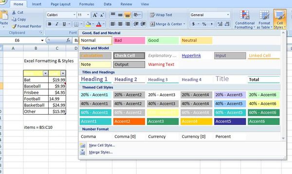
How to use Cell Styles in Excel?
Excel typically offers two efficient options to use cell styles on a selected cell or a range of multiple cells. We can either use any of the existing cell styles installed within Excel or create our custom style manually by choosing specific fonts, colors, shades, etc.
How is a cell style helpful in Excel?
Although cell styles in Excel are not as powerful as Word, they are helpful and save time to apply complex formatting within the sheet quickly. For example, consider that we have entered some data to around forty to fifty cells with the font size of 12 pt. But, later, we realized that we needed to use the font size of 16 pt. in all those cells instead of 12 pt. In such a case, we can edit the cell style and put the font of 16 pt., rather than editing the font size of each corresponding cell. All the cells with that specific style will automatically change to the font size of 16 pt.
How to Edit a Cell Style?
Excel also enables users to edit the cell styles as per their choice. We can edit our custom styles as well as the existing styles in Excel. For this, we need to go through the following steps:
How to merge or export cell styles from one Workbook to another?
Therefore, we need to merge cell styles to use the same style with other workbooks, which typically copies the applied style from one workbook to another .
What is a cell style in Excel?
Cell styles in Excel combine multiple formats. For instance, you might have a yellow fill color, a bold font, a number format, and a cell border all in a single style. This allows you to quickly apply multiple formats to the cells while adding consistency to the appearance of your sheet.
Can you share cell styles across workbooks?
When you’ve perfect ed your custom look, it’s easy to share cell styles across workbooks.
Is Excel a good program?
Excel does a good job of offering many premade cell styles that you can use. These cover everything from titles and headings to colors and accents to currency and number formats.
What is Excel format?
Excel allows us to format cells with predefined cell styles. These include different font sizes and styles, backgrounds, border styles, colors, etc. We’ll use the following data range with sales data to explain applying cell styles.
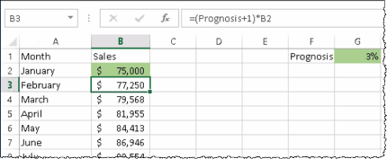
How to format range B3:E9?
Next, we can format range B3:E9 as input cells. In order to achieve this, (1) select the range. Then in the Ribbon, (2) go to the Home tab and in the Styles part, (3) click on More. In the offered menu, we’ll choose a cell style. In this case, we will use a style for input data: (4) Input. As a result, the range of cells B3:E9 is formatted as shown in the picture below.
How to format F3:F9?
Let’s (1) select the range, then in the Ribbon, (2) go to the Home tab and in the Styles part, (3) click on More. In the offered menu, we’ll choose a cell style. In this case, we will use a style for calculation data: (4) Calculation. As a result, the range of cells F3:F9 is formatted as shown in the picture below.